Ozone, UV and Aerosol studies
Total column water vapour
The absolute total amount of water vapour in a vertical column of air is named the total column water vapour (TCWV), the Integrated Water Vapour (IWV), or Precipitable Water Vapour (PWV or PW). The latter name refers to the fact that this amount could, hypothetically, precipitate out. Units are kg/m2 or mm (like rain). As the integrated water vapour is highly variable, both in space and time, measuring it remains a demanding and challenging task. Numerous techniques exist such as ground-based measurements, in-situ measurements (radiosondes) and measurements from space onboard satellites. All these techniques have their proper advantages and disadvantages (e.g. no measurements possible in the presence of clouds of rain), and their IWV retrievals have been inter-compared in numerous studies (see IWV inter-technique studies for a literature overview).
GNSS
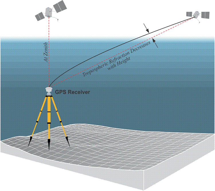
A signal between between a Global Navigation Satellite System (GNSS) satellite (of which the American Global Positioning System or GPS satellites were the pioneers) and a ground-based receiver is delayed along its path through the Earth's atmosphere by the ionosphere (a series of regions between 50 and 500 km that have a relatively large number of electrically charged atoms and molecules) and other "neutral" atmospheric layers. The ionospheric effects on the path delay can be eliminated using a combining of two GNSS frequencies. The remaining path delay depends on the integral effect of the densities of dry air, accounting for approximately 90% of the delay, and water vapour along the signal path. As one ground-based receiver can capture the time delays in multiple paths towards all GNSS satellites, those different "slant paths" between the receiver and the satellites are converted into the vertical direction (or zenith) by an elevation-dependent mapping function, hence resulting in a zenith total delay (ZTD) at the ground receiver site. As already noted above, also this measured zenith total delay can be reduced into two constituent parts: the zenith hydrostatic delay (ZHD, the dry part), and the zenith wet delay (ZWD, caused by the water vapour). Assuming hydrostatic equilibrium, the ZHD is easily modeled if the surface pressure is known. So, finally, the zenith wet delay is known (ZWD = ZTD - ZHD), and can then be transformed into integrated water vapour by making additional assumptions about the vertical temperature and humidity structure.
The major advantanges of retrieving integrated water vapour with GNSS is that it's an all-weather, high-precision, high temporal resolution (every 5 minutes), and relatively cheap technique. Moreover, time series at some GPS stations already date back to the middle of the 1990s. Drawbacks of the method are the relatively coarse global spatial resolution (with the highest density of GNSS networks in Europe and North America), the need for additional meteorological information, a consistent processing of the data during the entire time series, and the introduction of inhomogeneities due to e.g. hardware replacements (antennas and receivers), differences in the measurements (the number of visible GPS satellites and data rate) and in the environment (e.g. growing vegetation, different soil moisture). Homogenization studies to detect those inhomogeneities have already been undertaken, see e.g. Van Malderen et al. (2020).
IWV time variability and climate
Because of the intimate connection between changes in integrated water vapour (IWV) and surface temperature, described in the general section on water vapour, the assessment of the time variabililty of the IWV amounts in a warming climate is very attractive. As relatively long (since mid 1990s) IWV datasets from GNSS retrievals are available, these datasets can be used to validate IWV outputs from climate models, or to compare the IWV long-term variability with other IWV datasets or calculated from climate models.
We show two examples here. First we show in Fig. 2 the trends in integrated water vapour (in % per decade) for the period 1996-2014 for an European network of ground-based GNSS receivers (EPN), in comparison with the trends calculated from a merged satellite IWV product (GOMESCIA) and from a numerical weather prediction model reanalysis (ERA-Interim). Also included in the figure are the surface temperature trends from the same ERA-Interim model. We can observe that, globally, the IWV is increasing ("moistening atmosphere") over Europe, which aligns with the surface warming. However, there are differences in the IWV trends between the different datasets, especially between GNSS and the other two. This might be due to remaining inhomogeneities in the GNSS time series.

Fig. 2: Relative trends in integrated water vapour (in % per decade) for the period 1996-2014 from GPS (upper left), satellite instruments (upper right), and a climate model (lower left). The surface temperature trends (°C per decade) calculated from the same climate model are shown in the lower right panel.
We also calculated the IWV trends for the same datasets, but now for a the global International GNSS Service (IGS) network. These trends, again with the surface temperature trends, are shown in Fig. 3 below. We can again conclude that the IWV trends follow the surface temperature trends globally, with IWV trend differences between different datasets. In this case, the GPS and ERA-Interim trends are the most similar, with GOMESCIA deviating most from the other two.

Fig. 3: Relative trends in IWV (in % per decade) for the period 1996-2010 for the three different datasets as in the figure above, with the surface temperature trend (°C per decade) from ERA-Interim in the lower right panel.
To the literature overview of past IWV inter-technique comparisons (including GNSS)